ecoXCorr

ecoXCorr (pronounce “Eco-Cross-Corr”) is an R package designed to explore lagged associations between environmental time series and ecological or epidemiological responses based on the method proposed by Curriero et al. (2005)[1].

Table of content

• Introduction
• Installation
• Workflow overview
• Example
• Working with multiple independent time series
• One-step approach using the ecoXCorr() wrapper function
• References
• Licence

Introduction

It provides a coherent workflow to:

1. Aggregate environmental time series over multiple lagged time windows
   
2. Fit regression models across all lag structures
   
3. Visualize effect strength and direction using cross-correlation maps (CCM)

The package is particularly suited for studying delayed environmental effects, such as the influence of meteorological conditions on insect abundance or disease dynamics.

ecoXCorr shares several features with excellent climwin [2] package, but relies on glmmTMB, allowing to fit (generalized) linear mixed-models with a wide range of error distribution (including negative-binomial, zero-inflated, and zero-truncated; see ?glmmTMB::family_glmmTMB) as well as flexible covariance structures (see vignette(glmmTMB::covstruct)). The two packages also differ in their approach to multiple testing and error control. climwin addresses Type I error inflation through a simulation-based framework [2], whereas ecoXCorr controls for multiple testing using false discovery rate (FDR) adjustment of p-values. In addition, ecoXCorr provides greater flexibility in defining lag intervals, as these can be specified directly in numbers of days rather than being restricted to predefined time units (e.g. “week” or “month”), as in climwin. Conversely, climwin supports additional modelling frameworks that are not implemented in ecoXCorr, including cox proportional hazard model, multiple signal investigation, or weighted window models [2].

Below is an example of figure computed using ecoXCorr.

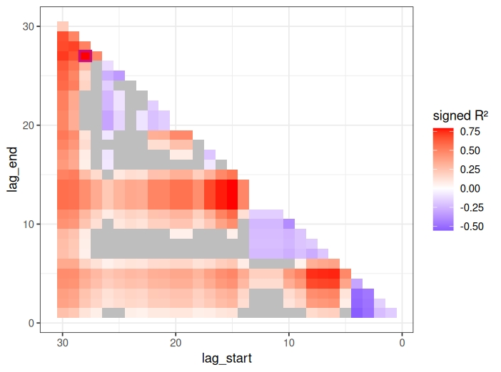
Fig. 1: Cross correlation maps showing the lagged effect of rainfall on Ae. albopictus abundance. Time lags are expressed in days prior to sampling. The signed R² reflects the variance explained by the explanatory variable, multiplied by the sign of the estimated effect. Pink-bordered square highlight the time lag with the highest R². Grey squares represent correlations with adjusted (for multiple testing) p-values > 0.05. Interpretation: mosquito abundance is best explain by rainfall recorded between 28 and 27 days before sampling.

When should I use ecoXCorr?

ecoXCorr is useful when:

• environmental drivers are expected to have delayed effects
• the relevant time scale of these effects is unknown
• you want a global view of lagged associations rather than testing a single lag

Typical applications include:

• variable and feature selection in modelling [4][5]
• vector ecology
• disease ecology
• environmental epidemiology
• climate–biology interactions

Installation

You can install the released version of ecoXCorr from CRAN with :

install.packages("ecoXCorr")

or the development version from GitHub:

# install.packages("devtools")
library("devtools")
install_github("Nmoiroux/ecoXCorr")

Overview of the workflow

The typical workflow in ecoXCorr follows three steps with respective functions:

1. Lagged aggregation of environmental data
   aggregate_lagged_intervals()

2. Model fitting across lag windows
   fit_models_by_lag()

3. Visualisation using cross-correlation maps
   plotCCM()

Steps 1 and 2 can be merged into a single step using the ecoXCorr() wrapper function.

The package ships with two example datasets to illustrate this workflow:

• meteoMPL2023: daily meteorological data (Montpellier, France, 2023)
• albopictusMPL2023: mosquito sampling data (Aedes albopictus, Montpellier, 2023)

The package includes a user-friendly Shiny application: ecoXCorrApp.

Example

Load required packages and example data

library(ecoXCorr)

# Meteorological daily time series
?meteoMPL2023
head(meteoMPL2023)

# Response data: tiger mosquito collections
?albopictusMPL2023
head(albopictusMPL2023)

Aggregate meteorological variables over lagged intervals

Meteorological variables are aggregated over all possible lag windows defined by:

• a reference date (d),
  
• a base interval length (i),
• a maximum lag (m)

For each reference date d, all intervals \([(d-1) - k \times i + 1; (d-1) - (l-1) \times i)]\) are generated, where i is the interval length (in days) and k, l range from 1 to m with k >= l.

In the example below i (interval) was set to 7 days, indicating that the unit for time intervals and lags will be a week. m (max_lag) was set to 8, indicating that the maximum lag (between response and predictor variables) considered will be 8 weeks (or \(m \times i\) days)

?aggregate_lagged_intervals

# get sampling days from our entomological dataset
sampling_dates <- unique(albopictusMPL2023$date)

# perform data aggregation for cumulated rainfalls and mean daily temperatures
met_agg <- aggregate_lagged_intervals(
  data       = meteoMPL2023,
  date_col   = "date",
  value_cols = c("rain_sum", "temp_mean"),
  ref_date   = sampling_dates,
  interval   = 7,               
  max_lag    = 8
)

head(met_agg)

Join environmental and response data

First check that response data has an ID unique identifier (if not, an ID field is created). ID field is required in the following step.

if (!("ID" %in% names(albopictusMPL2023))){
 albopictusMPL2023$ID <- rownames(ID)
}

Each observation (row in albopictusMPL2023), possibly on the same date, is associated with multiple lag windows, resulting in a many-to-many join:

data <- merge(albopictusMPL2023, met_agg, 
                by = "date", all = TRUE)

You might want to verify the resulting data set has the correct row number by multiplying the number of observations by the number of aggregation windows:

# Number of windows is the sum of integers <= `m` (max_lag parameter), which formulae is (with `m`=8):
n_windows <- 8*(8+1)/2
# expected number of rows in the resulting data frame:
expc_nrow <- nrow(albopictusMPL2023) * n_windows

expc_nrow == nrow(data)

Fit models across lag windows

Simple GLM example

Here, a Poisson GLM is fitted independently for each lag window:

?fit_models_by_lag

res_glm <- fit_models_by_lag(
  data       = data,
  response   = "individualCount",
  predictors = "temp_mean_mean",
  family     = "poisson")

Visualise results as cross-correlation maps

?plotCCM

plotCCM(res_glm, model_outcome ="R2sign", threshold_p = 0.2)

Each tile represents a lag window, with colour indicating the signed R² (% of variance explained × direction). Non-significant associations (p>0.2) are masked.

Other outcomes can be plotted (R², delta-AIC [3], Akaike weight [3], beta parameters of the linear predictor):

plotCCM(res_glm, model_outcome = "R2")
plotCCM(res_glm, model_outcome = "d_aic")
plotCCM(res_glm, model_outcome = "betas")

Mixed-effects model example

Because mosquito counts in the albopictusMPL2023 dataset are zero-truncated and observations are not independent (repeated measurements, spatial structure), a mixed-effects model may be more appropriate. This example illustrates how ecoXCorr supports such models:

?fit_models_by_lag

res_glmm <- fit_models_by_lag(
  data       = data,
  response   = "individualCount",
  predictors = "temp_mean_mean",
  random     = "(1|area/trap)",
  family     = "truncated_nbinom2")

plotCCM(res_glmm, model_outcome ="R2sign", threshold_p = 0.2)

The modelling function used depends on the random and family arguments:

• random is empty: stats::glm()
• random is specified OR family is a valid glmmTMB family: glmmTMB::glmmTMB()

Working with multiple independent time series

Not available with the current CRAN version

ecoXCorr can handle datasets containing multiple independent time series (e.g. from several stations) using the id_col argument in aggregate_lagged_intervals().

In this case, lagged aggregations are computed separately for each time series, ensuring that values are not mixed across groups.

Example

Here we artificially replicate the meteorological dataset to simulate two independent time series (e.g. two stations):

# Create two identical time series with different IDs
meteo_multi <- rbind(
  transform(meteoMPL2023, station = "A"),
  transform(meteoMPL2023, station = "B")
)

# Check structure
head(meteo_multi)

We then aggregate lagged predictors independently for each station:

sampling_dates <- unique(albopictusMPL2023$date)

met_agg_multi <- aggregate_lagged_intervals(
  data       = meteo_multi,
  date_col   = "date",
  value_cols = c("rain_sum"),
  ref_date   = sampling_dates,
  interval   = 7,
  max_lag    = 4,
  id_col     = "station"
)

The resulting dataset contains aggregated values for each station and lag window:

head(met_agg_multi)

You can then merge with a response dataset that also includes the same grouping variable:

# Example: replicate response data as well
albo_multi <- rbind(
  transform(albopictusMPL2023, station = "A"),
  transform(albopictusMPL2023, station = "B")
)

data_multi <- merge(
  met_agg_multi,
  albo_multi,
  by = c("date", "station"),
  all = TRUE
)

Finally, fit lagged models as usual:

res_multi <- fit_models_by_lag(
  data       = data_multi,
  response   = "individualCount",
  predictors = "rain_sum_sum",
  random     = "(1|trap)",
  family     = "nbinom2"
)

Key point

When id_col is used:

• lagged intervals are constructed within each group independently,
• no aggregation is performed across different time series,
• the output retains the grouping variable for downstream analyses.

This is particularly useful for multi-site studies with independent recording of environmental data.

One-step approach using the ecoXCorr() wrapper function:

This approach allows to plot CCM in one step giving one dataset of a meteorological time series and one dataset of response variable. Aggregation is performed for a unique time series (e.g. from only one station), a unique variable in the meteo dataset (argument value_cols) and according to a unique function (agg_fun). The resulting aggregated variable is used as the predictor in the modeling process.

?ecoXCorr()

res_glm <- ecoXCorr(
  meteo_data    = meteoMPL2023,
  response_data = albopictusMPL2023,
  date_col_meteo = "date",
  date_col_resp = "date",
  value_cols    = "rain_sum",
  agg_fun       = "sum",
  response      = "individualCount",
  interval      = 7,
  max_lag       = 8,
  shift         = 1,
  family        = "poisson"
)

References

Methods

[1] Curriero FC, Shone SM, Glass GE. (2005) Cross correlation maps: a tool for visualizing and modeling time lagged associations. Vector Borne Zoonotic Dis. doi:10.1089/vbz.2005.5.267

[2] van de Pol M, Bailey LD, McLean N, et al. (2016) Identifying the best climatic predictors in ecology and evolution. Methods in Ecology and Evolution. doi:10.1111/2041-210X.12590

[3] Burnham, Kenneth P., and David R. Anderson, eds. Model Selection and Multimodel Inference. Springer, 2004. https://doi.org/10.1007/b97636

Use cases

[4] Bartholomée C, Taconet P, Mercat M, Grail C, Bouhsira E, Fournet F, et al. Investigating the role of urban vegetation alongside other environmental variables in shaping Aedes albopictus presence and abundance in Montpellier, France. PLOS ONE. 2025;20: e0335793. doi:10.1371/journal.pone.0335793

[5] Taconet P, Porciani A, Soma DD, Mouline K, Simard F, Koffi AA, et al. Data-driven and interpretable machine-learning modeling to explore the fine-scale environmental determinants of malaria vectors biting rates in rural Burkina Faso. Parasites & Vectors. 2021;14: 345. doi:10.1186/s13071-021-04851-x

License

This package is released under the GPL-3 License.